Trade Area Analysis: Measuring Who Can Actually Reach You
A trade area is the geographic zone a location realistically draws customers from. How to build it with drive-time isochrones instead of radius circles, and how to enrich it into a full demographic and competitive profile.
You need to know how many customers can realistically reach each location, who they are, and whether nearby stores are competing with each other for the same people. That question has a name: trade area analysis.
A trade area is the geographic zone a location realistically draws customers from. Every business has one. Most haven't measured it. The shape of that zone determines your addressable market, your competitive exposure, and whether a new location nearby would grow revenue or cannibalize it.
This is the first in a three-part series on the GIS workflows that drive real business value, and it is the foundation for the other two. The polygons built here power the cannibalization check in site selection, and the territory logic behind route optimization.
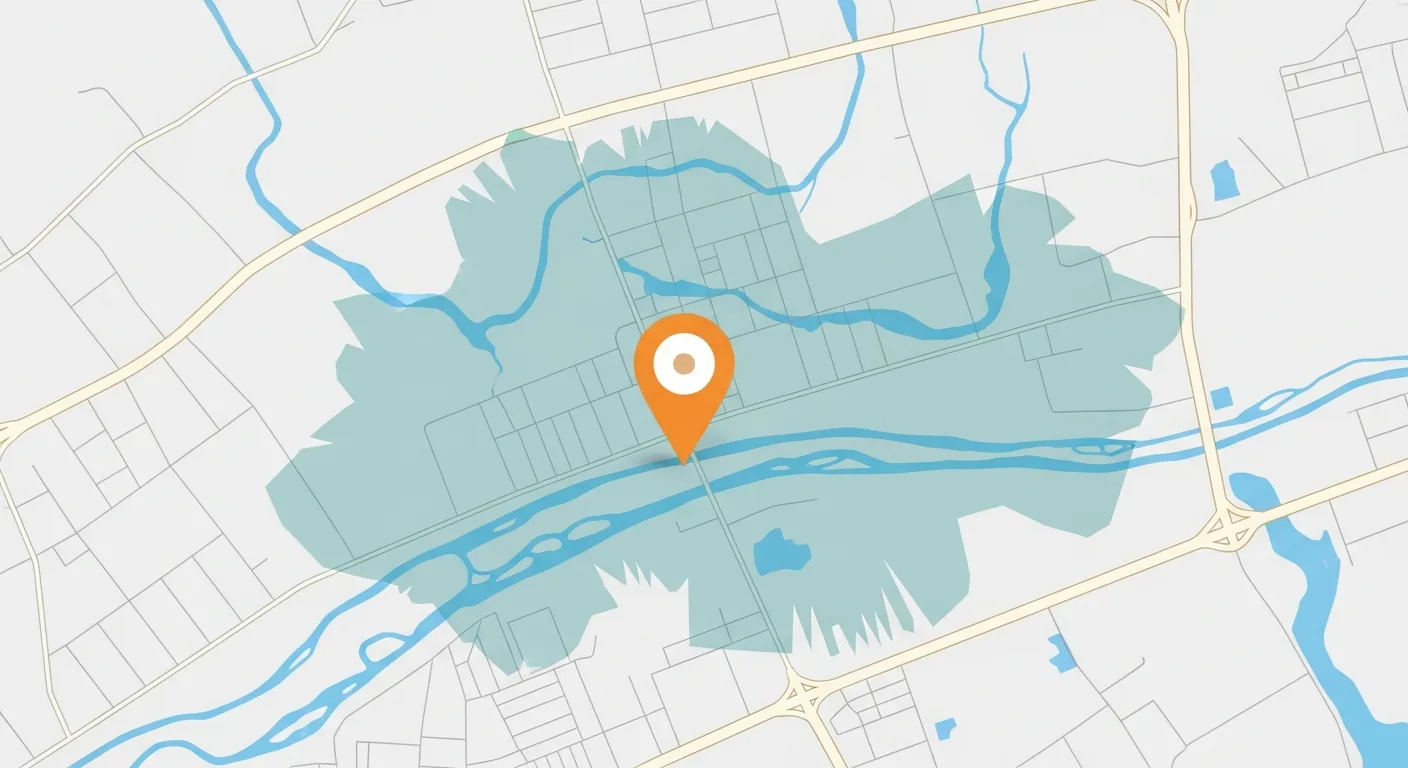
The key insight up front: the answer isn't a circle. It's a polygon shaped by the actual road network, drive times, not straight-line distance. Getting this wrong means overcounting people who can't reach you and undercounting people who can get to you fast via a highway.
What Trade Area Analysis Answers
The workflow shows up under different names in different industries, but the questions it answers are remarkably consistent.
- → What population can realistically reach this location?
- → What is the demographic profile of that population?
- → Where do competitors overlap with my coverage?
- → Does opening a new location grow revenue or just move it?
- → Retail: customer draw zones for each store
- → Distribution: delivery radius and service commitments
- → Healthcare: patient catchment and referral patterns
- → Financial services: branch coverage and ATM placement
Once the trade area polygon exists in your warehouse, answering the first question is a spatial containment check. Here is what that looks like in KQL, counting loyalty customers whose home falls inside each store's trade area:
One note on the shapes themselves: standard boundaries like counties and zip codes come ready-made, but sales territories and service zones do not. If your trade areas need to line up with internal business territories, you have to build those spatial assets yourself. That build process is the subject of The Spatial Supply Chain.
Radius Buffer vs. Drive-Time Isochrone
There are two ways to define a trade area polygon. One is fast and consistently wrong. One requires an API call and is worth every penny.
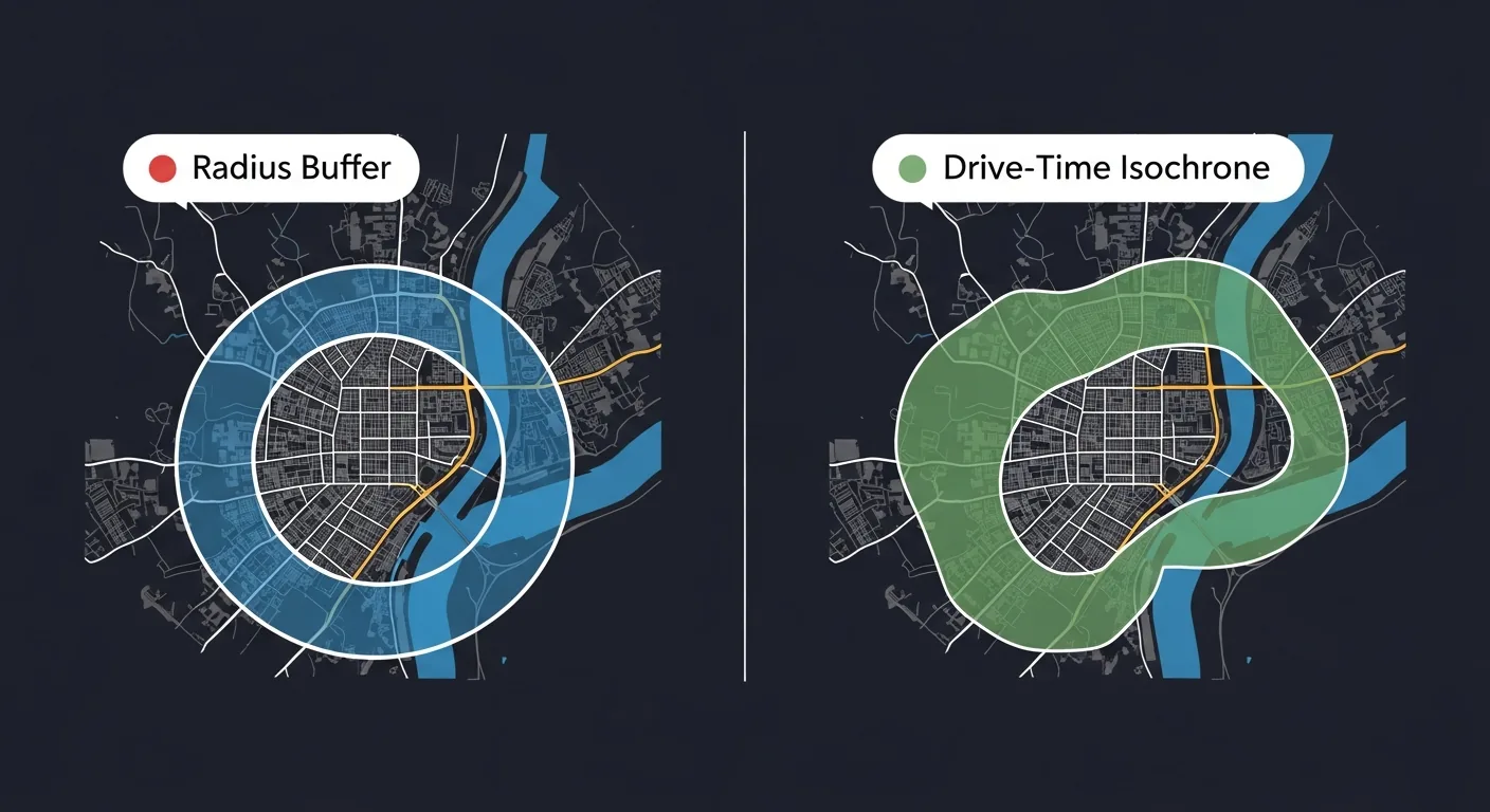
A circle of fixed radius centered on your location. Fast to compute, free to run, wrong by design. A 5-mile radius across a river includes thousands of people who need a 30-minute detour to reach you.
Use for: rough estimates in rural or sparse geographies where roads don't constrain movement meaningfully.
A polygon shaped by the actual road network. It expands along highways, shrinks around dead ends, and stops at barriers. Reflects how people actually travel.
The pattern: Call the Azure Maps or HERE routing API once in your ETL pipeline. Store the result as GeoJSON. Every downstream query reads the stored polygon: no live API calls at report time.
The architectural rule buried in that second card is the one that matters most in practice: isochrones are computed in ETL, not at query time. A routing API call costs money and takes hundreds of milliseconds. A stored polygon costs nothing to read. The MERGE pattern below refreshes stale isochrones on a quarterly cadence and leaves everything else untouched.
Enriching the Trade Area
The trade area polygon is the container. The value comes from what you spatially join to it. Each enrichment layer is computed once in ETL and stored as flat columns. By report time, every location has a full demographic and competitive profile with no geometry at query time.
The join mechanic here is worth pausing on: none of these datasets share a key column with your locations table. Geometry is the key. Using location itself as the join key across siloed datasets is the core idea in Location as the Universal Foreign Key.
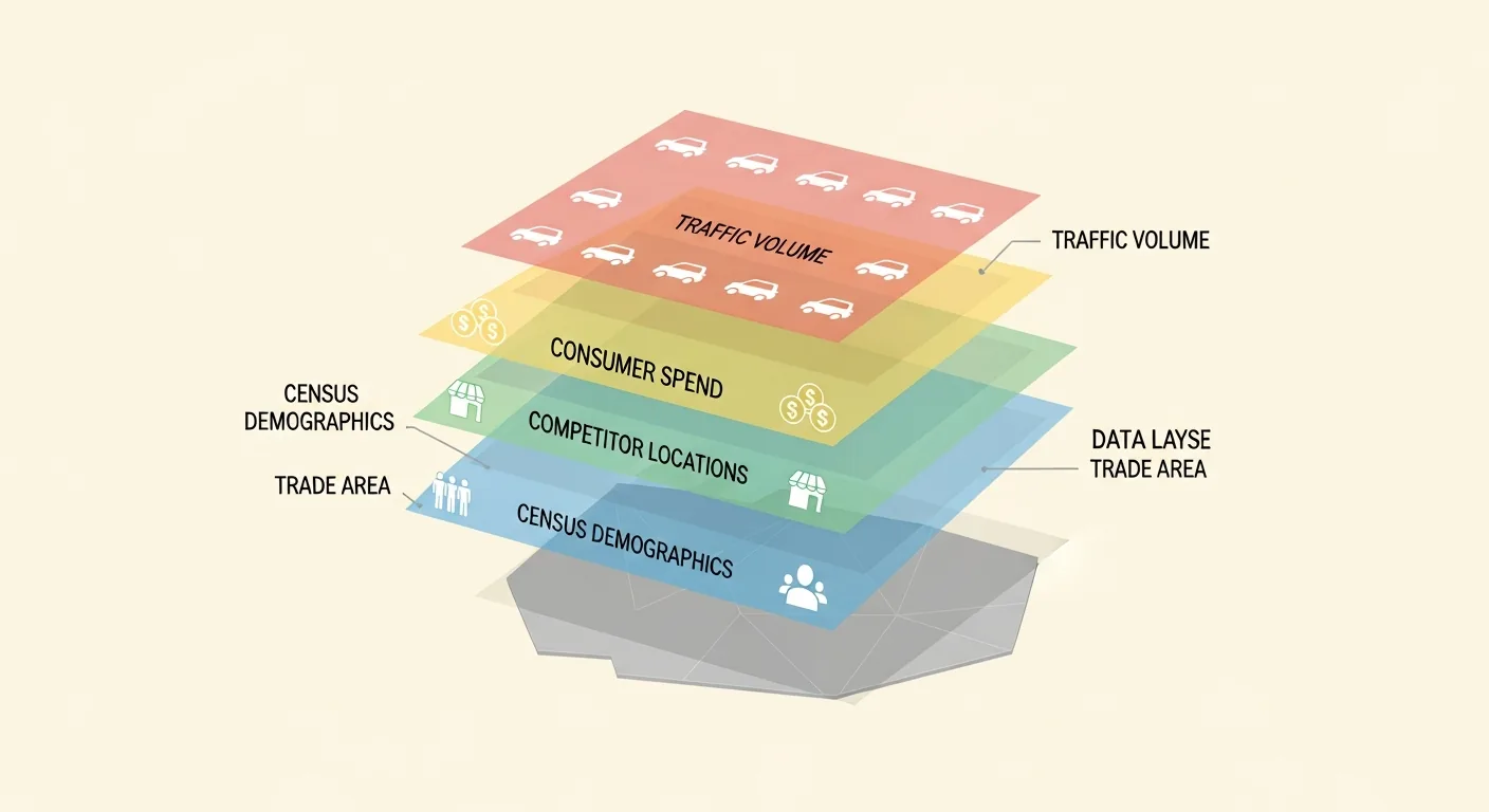
Population, median household income, age distribution, and household size, joined from Census block groups intersecting the polygon. The foundation layer for every scoring model.
Count, proximity, and brand of competing POIs within the trade area, sourced from SafeGraph, Precisely, or similar. Competitive density directly affects revenue potential.
Annual consumer spending in your category within the polygon, which signals total addressable market. Available from Esri, Experian, or derived from transaction data aggregators.
Daily average vehicle counts at nearby road segments from HERE or TomTom, a strong proxy for visibility and impulse traffic for locations that depend on passthrough customers.
The ETL that produces those flat columns is two spatial joins, aggregated separately. Joining block groups and competitors in a single query multiplies the rows before aggregation. Every population sum gets inflated by the number of competitor matches. Two CTEs keep each aggregate honest:
One honest caveat on that demographics CTE: ST_Intersects claims a block group's entire population the moment the trade area clips any part of it, so a polygon that catches five percent of a large suburban block group inherits one hundred percent of its people. That is fine for a first-pass profile and wrong for anything you put in front of a real estate committee. The fix is areal interpolation: apportion each block group's counts by the share of its area falling inside the polygon. This is covered end to end in enriching trade areas with Census demographics. The AVG(bg.MedianIncome) above has the same problem twice over, since medians do not average.
Where This Leads
An enriched trade area is useful on its own: it tells you the addressable market and competitive exposure of every location you already operate. But its highest-leverage use is downstream. When you evaluate a new candidate site, overlapping its projected trade area against your existing ones is the difference between growing the network and quietly redistributing it. That check, cannibalization analysis, is where site selection picks up.