Route Optimization Is Mostly a Visibility Problem
The optimizer already exists in your TMS or scheduling tool. What most organizations are missing is the observability layer: storing planned routes and actual GPS traces so you can see where the plan breaks down.
People and vehicles move between stops all day, and every extra mile costs fuel, drive time, and missed service windows. Yet most organizations don't have a routing problem. They have a visibility problem.
The optimizer already exists, in the TMS, the logistics platform, or the scheduling tool. Fleets commonly report 10 to 20 percent fuel savings just from moving off manual dispatch to an optimizer, before any behavior change. What's missing in most organizations is the observability layer that shows where the optimized plan is followed and where it breaks down. Building that layer is the BI team's job, and it is the subject of this article.
This is the second in a three-part series on the GIS workflows that drive real business value, alongside trade area analysis and site selection. All three read from the same spatial data model.
The workflow applies anywhere a person moves between locations: last-mile delivery, field service technicians, sales territory coverage, medical equipment servicing. The math is the same: a weighted search problem constrained by time, capacity, and regulation.
Which driver visits which stops in what order. Constrained by vehicle capacity, customer time windows, and HOS driving regulations.
Which technician covers which service calls. Matching requires skill compatibility, appointment windows, and travel time between sites.
Dividing a region so reps spend time selling, not driving. Balances stop count, drive time, and account tier across the team.
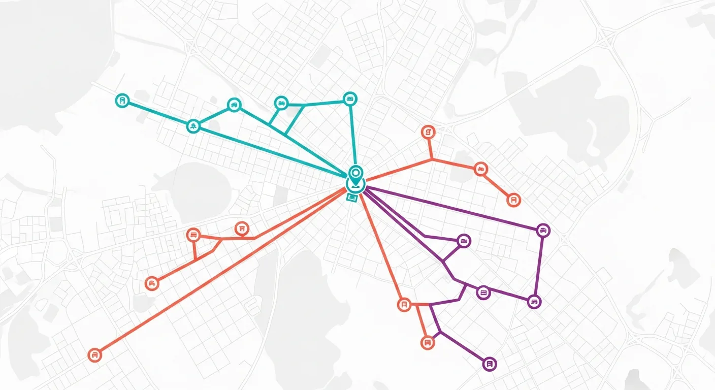
Whatever solver you use, its core input is a cost matrix: the drive time between every pair of stops. Like the isochrones in trade area analysis, this is computed once in ETL via a routing API and stored, never called live at query time:
Planned vs. Actual: The Observability Gap
A common failure mode: the optimizer ran correctly, and the driver ignored the sequence. Without storing both the planned route and the actual GPS trace, you have no way to know this happened, or to measure the cost.
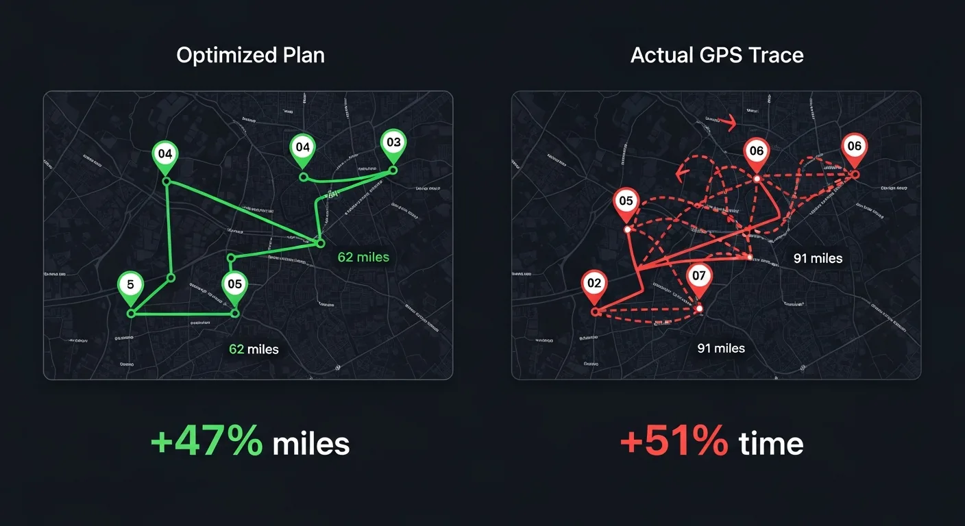
In this example, the optimized plan was 62 miles and 4.1 hours. The actual GPS trace was 91 miles and 6.2 hours: the driver went to Stop C first, then backtracked to Stop A, adding 29 miles and over two hours. This is the BI team's deliverable: a Power BI report comparing planned vs. actual by driver, territory, and day.
- → Planned route as a LineString geometry in your warehouse
- → Planned stop sequence and time windows
- → Actual GPS trace from the TMS or device
- → Actual arrival times at each stop
- → Miles vs. planned: the route adherence ratio
- → Time vs. planned: on-time rate by stop and driver
- → Sequence deviation: stops visited out of order
- → Missed time windows: late arrivals by priority tier
With both sides stored, the adherence metrics fall out of a single query. This KQL computes the adherence ratio and sequence drift for every route in the last week, and flags anything running more than 15 percent over plan:
The Vehicle Routing Problem
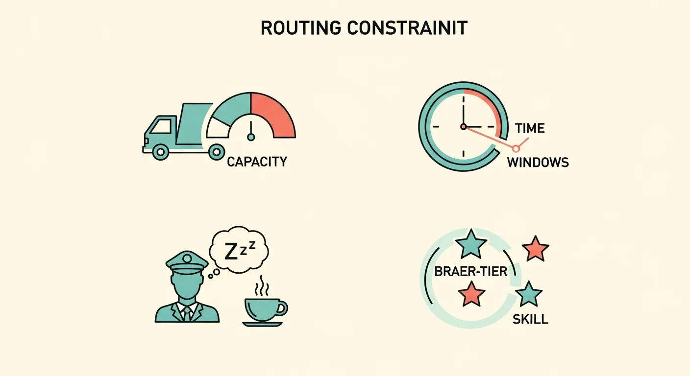
It helps to understand what the optimizer is actually solving, because it explains why "the plan looks wrong" complaints are usually the plan being smarter than intuition. Real-world routing isn't "find the shortest path." It's a constrained optimization problem that grows exponentially with every constraint added. Most solvers use heuristics; exact solutions stop being practical past a few dozen stops.
-
1. Multiple vehicles with capacity limits
Each vehicle has a weight or volume ceiling. Adding K vehicles doesn't divide complexity by K; it multiplies the search space. Stops must be assigned so no vehicle exceeds its limit.
-
2. Time windows at each stop
Customers want delivery between 9 and 11am, or between 2 and 4pm. The sequence must respect clock constraints, not just distance. A missed window means a re-delivery: pure cost, zero revenue.
-
3. Driver shift hours and mandatory breaks
HOS regulations require mandatory rest breaks at set intervals. Routes must be structured so break points line up with geography; you can't take a break mid-delivery at a customer site.
-
4. Priority tiers and SLA penalties
The optimizer minimizes a weighted cost function, not just distance. Lateness for a Priority 1 customer carries a 10x penalty vs. Priority 3, so the sequence puts SLA ahead of pure efficiency for key accounts.
The data team's contribution here isn't building the solver. It's surfacing the stops the solver can't feasibly serve, before dispatch, so a human resolves them instead of a driver discovering them on the road:
Where This Leads
Store planned routes as LineString geometry, load the GPS traces next to them, and the variance layer becomes an analytical question rather than an engineering project. The same territory boundaries that structure your routes also tell you where coverage is thin, which is one of the signals that feeds site selection. And the polygons that define those territories are custom spatial assets you build and maintain, the process covered in The Spatial Supply Chain.