Geofencing for Marketing in Microsoft Fabric
How to build a competitor visit detection and proximity marketing system using Azure Maps and Microsoft Fabric, from fence definition to audience activation. Told through a real-world scenario.
A geofence is a virtual boundary drawn around a real-world location. When a customer's device crosses that boundary, you know, and you can act on it in seconds. For marketing teams, this is the closest thing to reading a customer's mind: they just walked out of a competitor. What do you do next?
This article covers how to build that system on Microsoft Fabric, using Azure Maps as the spatial engine. The first half is the architecture: the services, the pipeline, the data model. The second half follows a fictional retail brand, Meridian Coffee, as they build a competitor visit detection campaign from scratch, step by step. Because Meridian is fictional, every metric in its story (conversion rates, dwell times, visit frequencies) is illustrative, there to show the shape of the analysis rather than report real campaign results.
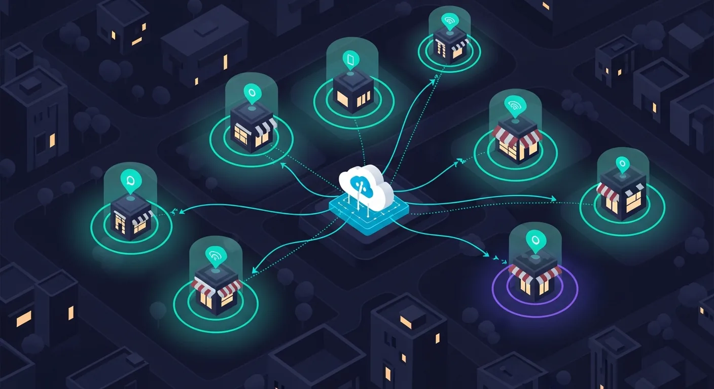
- 3x higher conversion on proximity-triggered offers. vs. time-based campaign blasts with no location context.
- Under 90 s latency from geofence exit to offer delivery. With Fabric Eventstream + KQL real-time matching. Time window matters: the offer has to arrive before they reach their car.
- 4 Azure Maps services in this stack. Geofencing API, Search API (address and footprint data), Route API (drive-time zones), and Maps Render for Power BI.
The Three Marketing Use Cases
Before building anything, be precise about what you're building. Geofencing for marketing collapses into three distinct patterns, each with a different latency requirement, a different trigger, and a different activation target.
The Azure Maps + Fabric Architecture
Four services do the work. Azure Maps owns the spatial layer: fence definitions, real-time event detection, and drive-time zone generation. Fabric owns the data layer: ingestion, storage, transformation, and reporting.
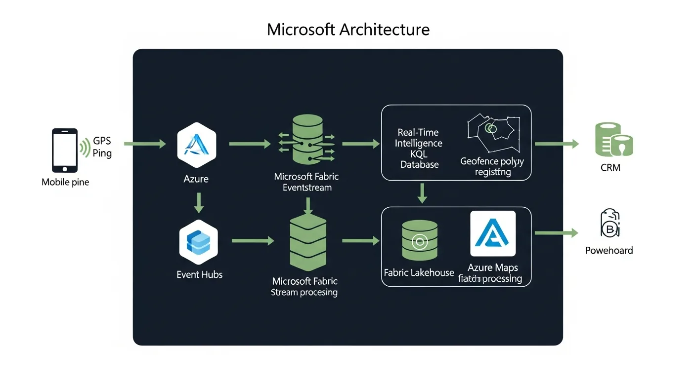
- → Geofencing API: submit a coordinate plus your fence geometries, get back each fence's signed distance (negative = inside). Stateless, low-latency, REST. You derive ENTER/EXIT by comparing consecutive results.
- → Fence storage: you store the fence GeoJSON yourself (here, in the Lakehouse) and send geometries in the Geofencing request body. Azure Maps Creator's dataset-upload workflow was retired in September 2025.
- → Route API: generate drive-time isochrones used as fence boundaries when you want "reachable in 10 minutes" not a fixed radius.
- → Eventstream: ingest mobile location events from Azure Event Hubs. Fan out to KQL and Lakehouse simultaneously.
- → Real-Time Intelligence / KQL: geospatial join between live location events and fence geometries. Sub-second matching.
- → Lakehouse (Delta): persistent store for all historical events, fence crossings, dwell times, and audience segments.
The Ingestion Layer: Eventstream
Location events arrive as a stream: each event is a device ping with a coordinate, a timestamp, and a user identifier. The mobile app sends these to Azure Event Hubs; Fabric Eventstream picks them up and routes them to two destinations simultaneously: a KQL Database for real-time matching and a Lakehouse Delta table for the historical record.
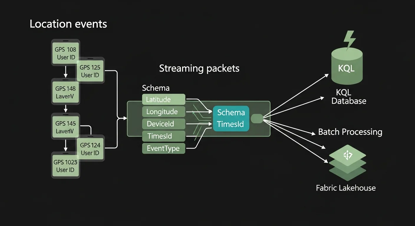
One configuration decision matters more than any other: filter out low-accuracy pings before they reach the matching engine. Indoor GPS drift is real: a customer sitting in a competitor café can register as inside your fence 80 metres away. Add the accuracy filter in the Eventstream transform step, not downstream.
Real-Time KQL vs Batch Spark: When to Use Which
The matching engine choice depends entirely on your latency requirement. If the offer has to arrive within 90 seconds of the fence crossing, you need KQL. If you're building weekly audience segments for email campaigns, Spark in the Lakehouse is simpler and cheaper.
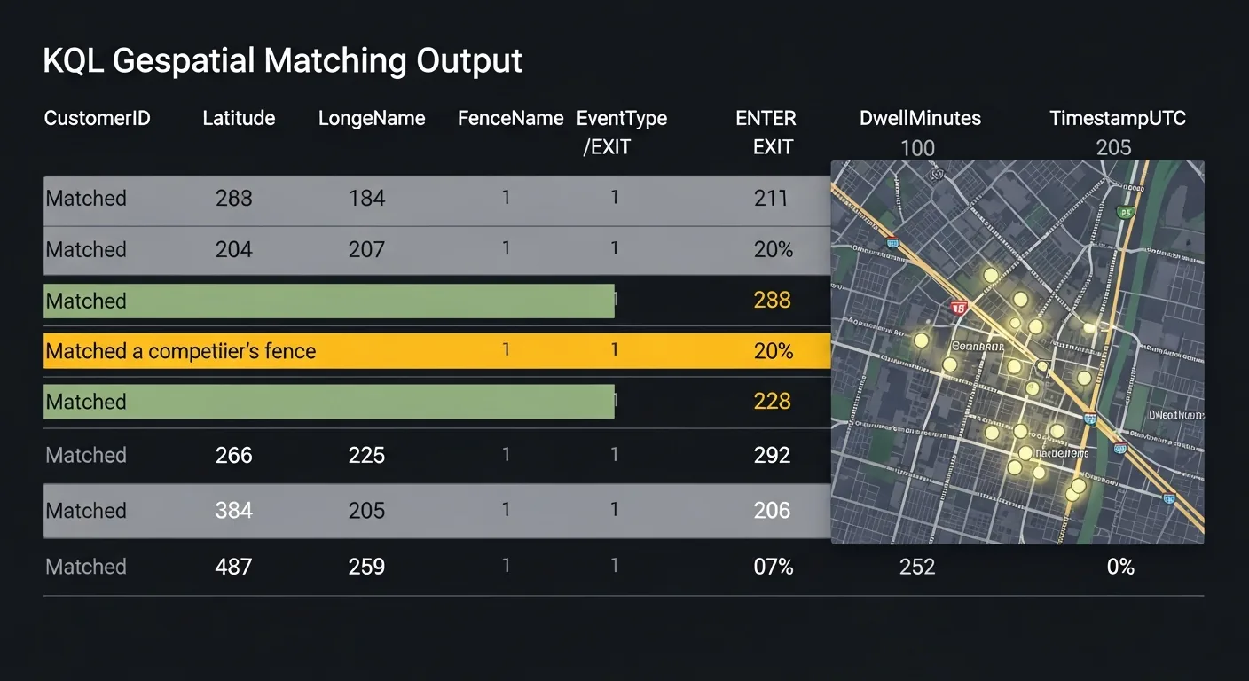
- → Latency requirement is under 2 minutes
- → Trigger is a single event (enter/exit)
- → Activation is a push notification or webhook
- → Building daily or weekly audience segments
- → Dwell threshold required (>10 min)
- → Activation is CRM sync, email batch, or paid media
The Meridian Coffee Story
Everything above is the architecture. What follows is what it looks like to actually build it: decisions made, queries written, segments created. We're following the data team at Meridian Coffee, a regional specialty coffee chain with 34 locations, as they build their first competitor visit detection campaign.
Meridian's head of marketing noticed something in their customer data: loyalty app users who visited a competitor location in the previous 30 days had a 23% lower visit frequency in the following 30 days. The question wasn't whether competitors were affecting retention. It was whether Meridian could catch the defection signal in real time and do something about it before the customer formed a new habit.
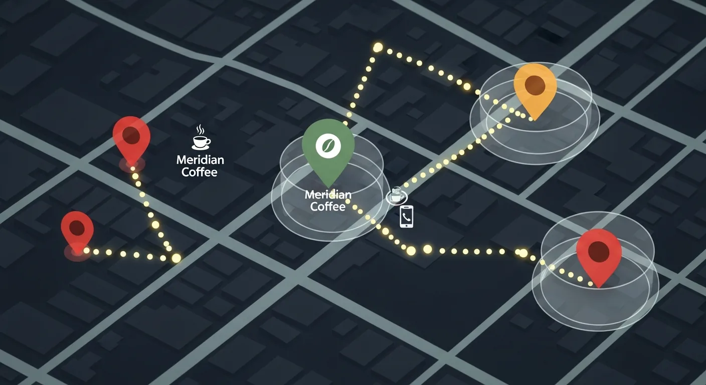
Step 1: Draw the Fences
The data engineer started by pulling a list of every competitor location within 1.5 miles of a Meridian store: 47 locations across 5 competitor brands. For each one, she drew a 100-metre geofence polygon fitted to the building footprint, using the Azure Maps Search API to get address and footprint data, and stored it as GeoJSON in the Lakehouse.
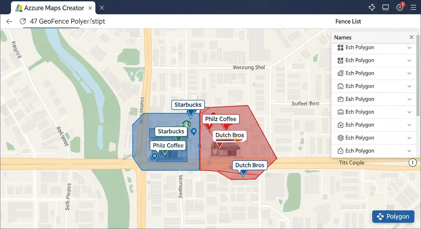
The Lakehouse geofences table is the source of truth: the enrichment Function loads the active fence geometries from it and sends them in the Geofencing API request body at runtime, and the same table feeds the Spark batch path and Power BI reporting.
Step 2: Wire the Eventstream
The loyalty app was already sending anonymised location pings to an Azure Event Hub every 30 seconds when the app was in the foreground. The data engineer created a new Fabric Eventstream, pointed it at that Event Hub as the source, and added two destinations: the KQL Database for real-time matching, and a Lakehouse Delta table for the historical record.
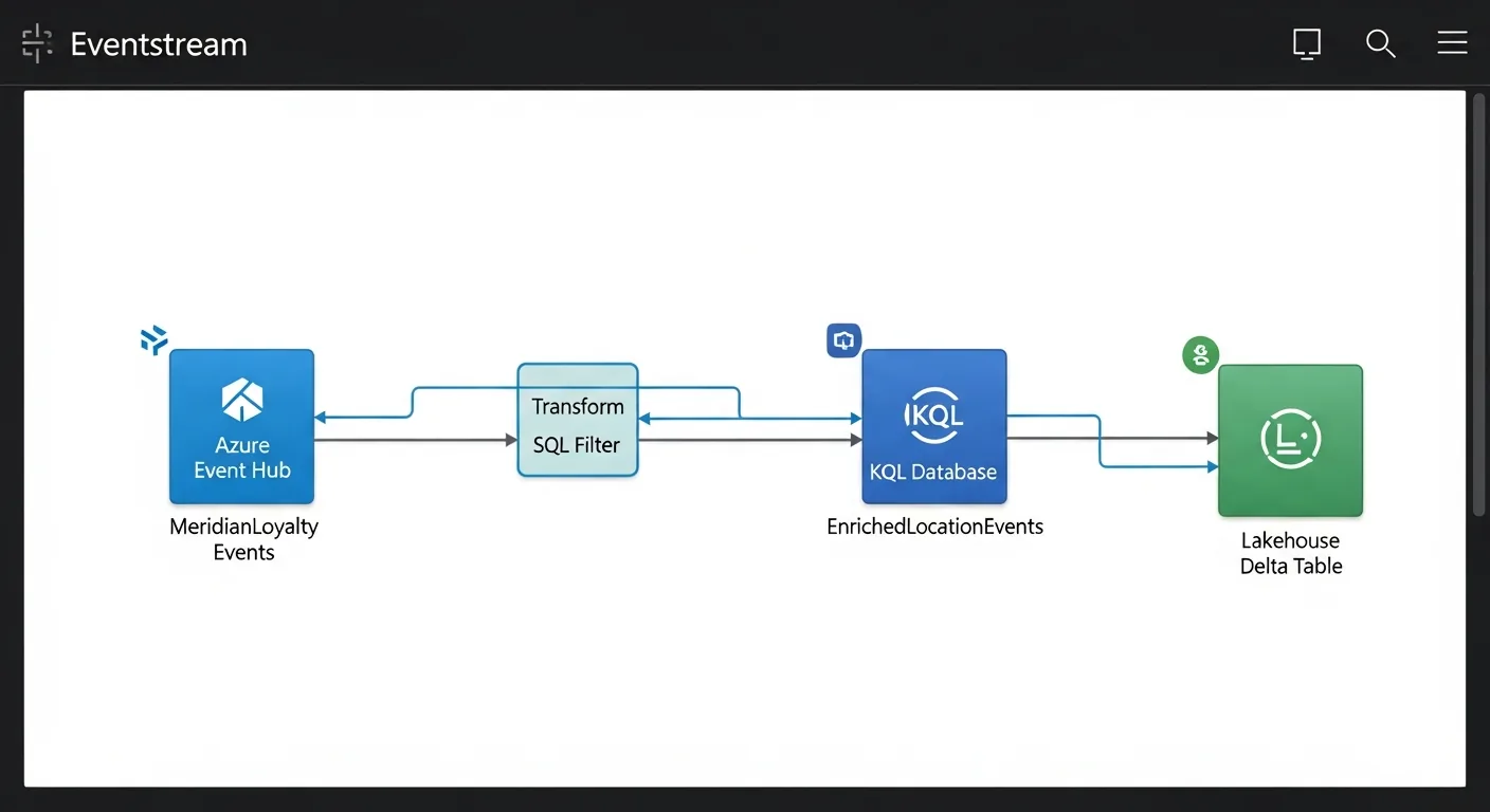
One important configuration: she added a filter in the Eventstream transform step to drop events where accuracy_metres > 50. Indoor GPS drift near competitor locations created false positives in testing. The filter eliminated nearly all of them.
Step 3: The KQL Query That Catches the Visit
Eventstream transforms can filter and reshape events, but they can't call external APIs, so a small Azure Function sits between the Event Hub and the Eventstream. It calls the Azure Maps Geofencing API for each location ping and emits the enriched event onto the stream. The API returns which fences matched. The enriched event that lands in KQL already contains FenceId and Brand from the API response. The KQL query then summarises entry and exit times per customer per fence, applying a 3-minute dwell threshold to eliminate drive-bys.
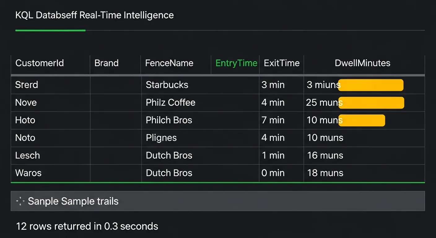
A customer who genuinely visited a competitor spent at least 3 minutes inside the polygon. That's a real signal. A ping at 45 seconds is noise, and if you activate on noise, the offer feels random and undermines trust in your loyalty programme.
Step 4: Write the Audience Segment
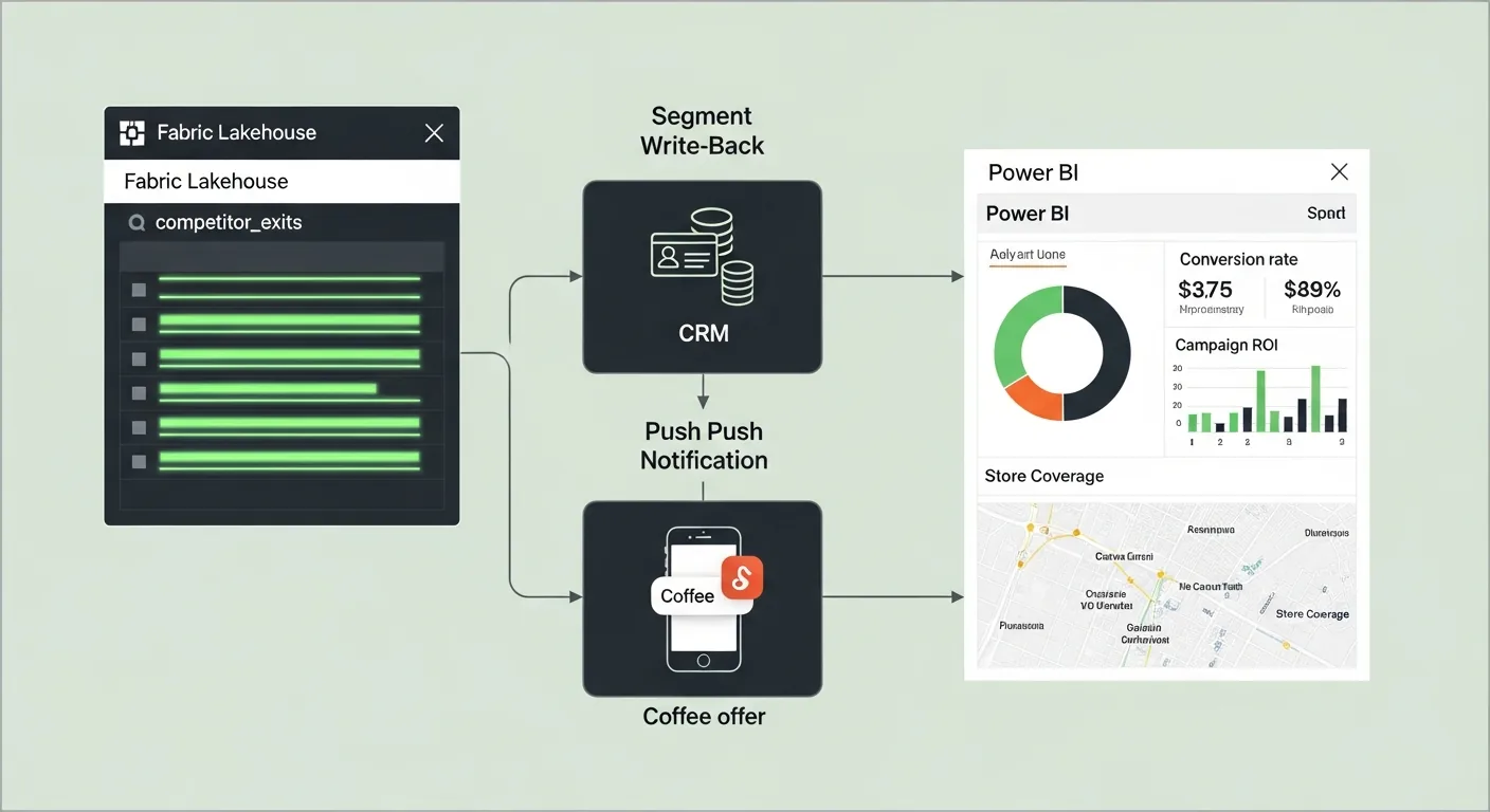
Confirmed competitor exits land in the KQL competitor_exits table. A Fabric Activator rule watches that table and fires a webhook to Dynamics 365 CRM whenever a new row lands. The CRM queues a personalised push notification (a free drink offer valid for 4 hours), sent via Azure Notification Hubs.
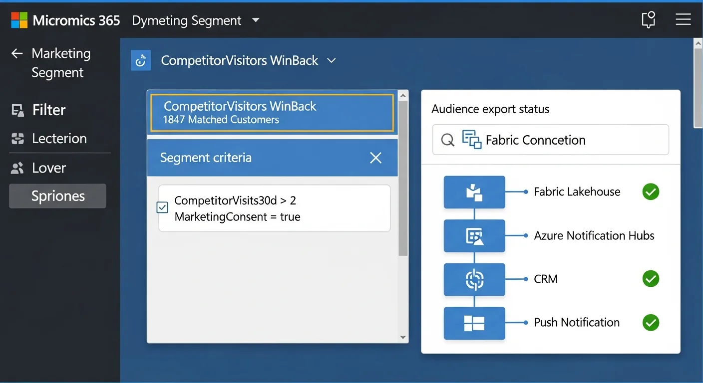
For the weekly email path, a Spark notebook runs nightly against the Lakehouse, builds the audience segment from 30 days of exit history, and syncs to the CRM via the Dataverse connector. Same data, different cadence, different channel. The Lakehouse is the single source of truth for both real-time and batch activation.
Step 5: The Power BI Report
The marketing team needed a single report to answer three questions: which competitor locations are pulling the most customers, how long are customers staying (dwell time), and what is the win-back campaign converting at. All three answers live in the same Lakehouse Delta tables. The report is a read-only view over data the pipeline already produced.
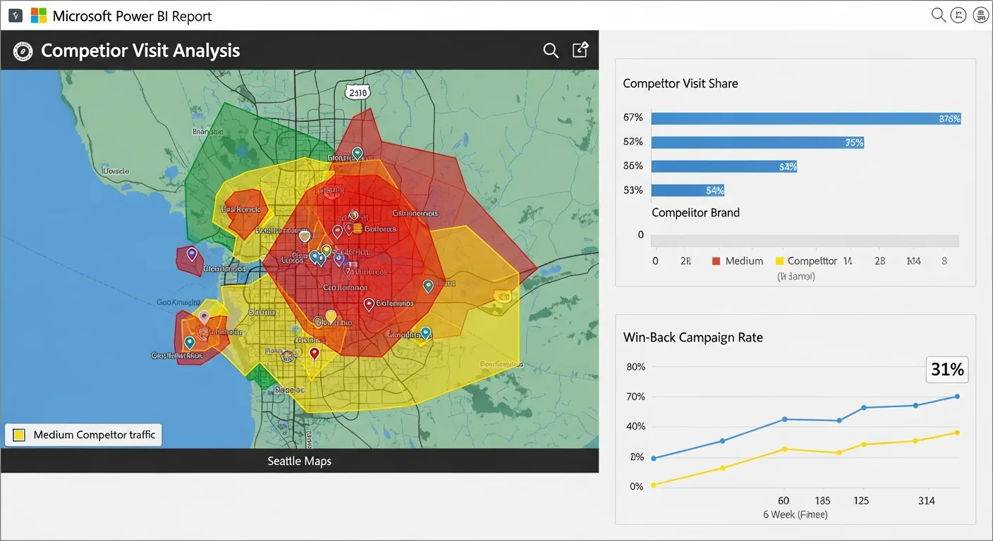
The Azure Maps visual in Power BI renders each competitor fence as a polygon layer, coloured by visit count, giving the marketing team an instant geographic read on where the competitive pressure is highest. The Azure Maps Render service handles the tile layer; the Lakehouse handles the data.
What Meridian Learned
Six weeks after launch, the first read-back was clear: customers who received a win-back offer within 90 seconds of exiting a competitor converted at 31%, nearly three times the 11% rate of the control group who received the same offer the following morning. The latency window was the variable that mattered most.
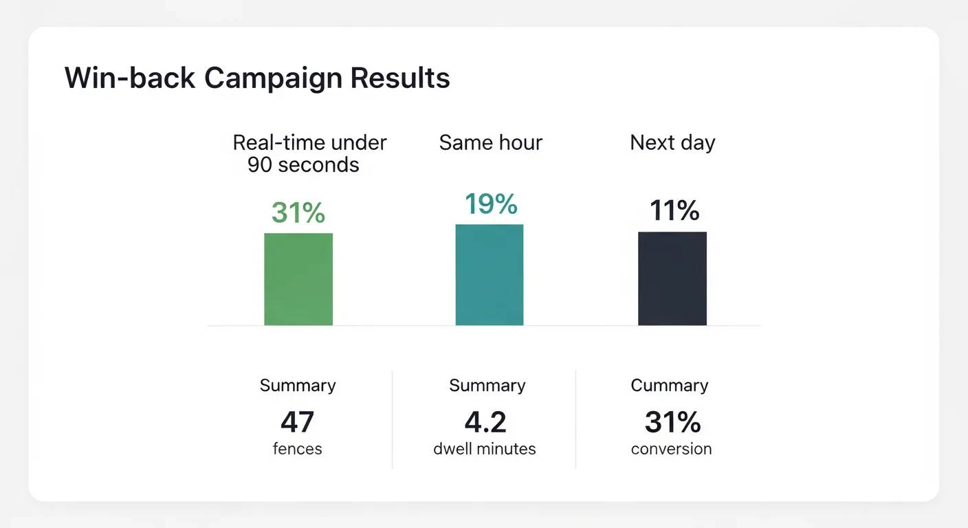
- 31% conversion on real-time win-back. Delivered within 90 seconds. Control group (next morning): 11%.
- 4.2 avg dwell minutes before exit trigger fires. The 3-minute dwell filter proved correct: events below it had near-zero conversion.
- 47 competitor fences across 5 brands. All stored as GeoJSON in the Lakehouse: versioned, queryable by KQL and Spark, and sent to the Geofencing API at runtime.
The three things that made it work: The dwell-time filter: without the 3-minute threshold, drive-bys flooded the segment and the offer felt random. The 90-second activation window: the offer arrives while the customer is still in the decision state. And consent: Meridian's loyalty app had explicit location consent at signup. This entire pipeline was built on opt-in data. That's not just a legal requirement; it's what makes the offer feel personalised rather than surveilled.